Guidance on using an updated collision risk model to assess bird collision risk at onshore wind farms
Published: 2024
1. Introduction
An environmental statement for an onshore wind farm should include a quantitative estimate of collision risk for all bird species present on the site for which the level of risk has the potential to be important. This should include a view on the significance of that collision risk to the respective bird populations.
The aim of this guidance is to promote a standardised approach to collision risk assessment for onshore wind farms, to increase the transparency of calculations and to promote greater confidence in the results. It will enable estimates from different wind farms to be more easily compared and combined to facilitate cumulative assessment. It may also enable collision risk assessment to be used as a tool in selecting the best areas for onshore wind farm development.
The guidance describes the information needed, and how to use that information to arrive at an estimate of collision risk. It is accompanied by a spreadsheet which enables the necessary calculations to be performed in a standardised way.
The approach builds on previous models developed by Band et al. (2007) and Band (2000). The approach does not change the single transit probability calculation but adds the other stages of the model, which would previously have been undertaken by consultants and others wishing to conduct collision risk modelling, to standardise these calculations. The approach is intended to provide collision risk estimates that are comparable across different wind farms.
This guidance provides an explanation of the model input parameters, how the information should be presented and how the outputs of the model should be expressed. . It is associated with a spreadsheet for performing the calculations. A fuller report is available explaining the derivation of the model (Band, 2024).
2. Information needed
The model requires information on:
- The number of birds flying through or around the site, and their flight height (derived from bird survey).
- Any predicted or likely changes of behaviour of birds, e.g. in avoiding or being attracted to the wind farm.
- The number, size and rotation speed of turbine blades.
- Physical details on bird size and flight speed.
Figure 1 illustrates graphically the process involved. The guidance does not cover:
- bird survey methods - for which there are various advisory sources, notably our guidance Survey methods for use in assessing the impacts of onshore windfarms on bird communities; or
- bird behaviour – which can be obtained from other guidance, such as our guidance Use of avoidance rates in the NatureScot wind farm collision risk model.
The key outputs from the collision model – the collision risk - is expressed as the likely number of birds per month or per year which will collide with the wind farm. It should include the range of uncertainty surrounding that estimate. Presentation of the output should be accompanied by a clear statement of the assumptions on avoidance made in arriving at the estimate as these are often critical to the magnitude of the collision estimate.
The model provides only an assessment of collision risk. Where collision risk is estimated to be not negligible, a developer will need to consider the significance of the predicted mortality. This will include the sensitivity of the bird population, the degree of protection afforded by legislation and any protected sites in the vicinity which may be designated for that species by legislation and any protected sites in the vicinity which may be designated for that species.
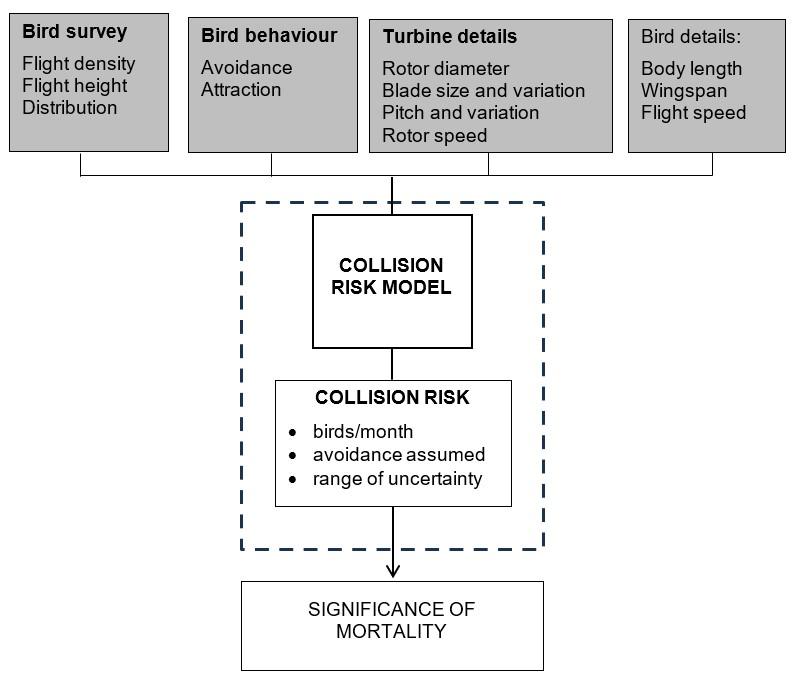
Figure 1. Collision risk model process. Grey boxes require a standard presentation of information.
Click for a full description
Figure 1 is a flow chart describing model inputs and outputs. Input data is on bird behaviour, i.e. avoidance or attraction to the site, bird survey, i.e. flight density, height and distribution, turbine details, i.e. rotor diameter, blade size and variation, blade pitch and variation and rotor speed, and details of the bird species, i.e. their body length, wingspan and flight speed. Data is analysed in terms of the number of birds per month, avoidance behaviour and an assumed range of uncertainty, and the output results presented as the significance of the risk of mortality occurring. Input data needs to be in a standardised form to allow the calculations to be made accurately.
3. Collision risk model
The model estimates the number of collisions through a process of five stages:
- Stage A uses bird survey data to establish the density of flying birds in the vicinity of the turbines, and the proportion flying at a risk height, between the lowest and highest points of the rotors.
- Stage B provides an estimate, based on the bird density and proportion at risk height, of the potential number of bird passages through rotors in the period in question.
- Stage C calculates the probability of collision during a single bird rotor transit.
- Stage D estimates the potential collision rate for a bird species, assuming current levels of bird use of the site, allowing for the proportion of time that turbines are not operational.
- Stage E takes account of the proportion of birds likely to avoid the wind farm or its turbines, either because they have been displaced from the site or because they take evasive action or are attracted to the wind farm, e.g. in response to changing habitats.
Thus, expected collisions =
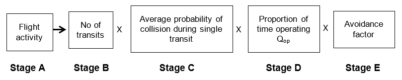
Figure 2. The collision risk model stages.
Click for a full description
Figure 2 is a flow chart presenting the five stages of the model. Data in flight activity is used to estimate the number of single transits through the rotor area, the average probability of collision during each of these transits, then multiplied by the proportion of the turbine operational time (Qop) and the avoidance factor.
The guidance describes each of the five stages. It includes an additional stage, Stage F, which describes how to express the uncertainty surrounding a collision risk estimate.
4. Collision risk model spreadsheet
This guidance is carried out using a spreadsheet which enables user to work easily through stages A-E of the process. It comprises five worksheets.
Collision risk. This is the ‘master’ spreadsheet into which all required data is entered (except blade profile), and which presents the collision risk output. An illustration of this spreadsheet, as used for the worked example, is reproduced at Annex 1.
Data is entered in the top section of the spreadsheet. It is brigaded under three headings: ‘Bird data’, ‘Wind farm data’ and ‘Turbine data’. The only data which requires input elsewhere is in the ‘Blade profile’ sheet where, if the data is available, the blade profile may be replaced by a more specific one for the turbine blades used.
The remainder of the sheet is organised according to Stages A-E of the process. It provides outputs from each stage:
- Stage A – the calculated flight activity (expressed as a density figure).
- Stage B - the estimated number of potential bird transits through rotors of the wind farm.
- Stage C - the probability of collision during a single bird rotor transit.
- Stage D - potential collision mortality for the bird species, assuming current use of the site and no avoiding action is taken.
- Stage E - potential collision mortality for the bird species, taking avoidance and other likely behaviour change into account.
The source data used for each input should be listed in full within the environmental statement.
Blade profile is a table giving the chord width of the blade, relative to its maximum chord width, at points along the blade length. 21 data points are required, at points r/R = 0, 0.05, 0.1, 0.15 etc. up to r/R=1 where r is the distance out from the hub and R is the blade length. The value for r/R=0 is not used in the calculation as this will be the hub.
Daylight and night hours. Given the input latitude, this sheet computes the daylight and night hours in each month within which there could potentially be bird activity.
Large array correction. This enables a correction to be made for large arrays where the collision rate is such that bird density might significantly decline as birds pass through the wind farm. These correction factors are then applied to the collision rate estimates in the ‘Collision risk’ sheet. In most circumstances the results will demonstrate that a large array correction is not significant and can be ignored.
Spreadsheet protection
The spreadsheet uses visual basic functions to calculate collision risk for single transits. For these to work, the spreadsheet must be macro-enabled. Some corporate systems routinely disable macros as a computer security precaution. These can be enabled in File/Options>Trust Center>Trust Center>Settings>Macros Settings and activating ‘Enable all macros’.
To protect against unintentional overwriting of formulae, or the entry of input data other than in the ‘Collision Risk’ sheet, each of the worksheets is protected. The spreadsheet is fully usable in this state, with data entry allowed in the sections coloured orange.
5. Stage A - Flight activity
This stage estimates the number of flights which, in the absence of birds being displaced, taking other avoiding action or being attracted to the wind farm, would potentially be at risk from the turbines. It requires field data to determine levels of flight activity within the proposed wind farm.
For non-directional flights, two key parameters derived from survey observations are needed to describe the magnitude of flight activity:
(i) Areal bird density (DA) and
(ii) Proportion of birds flying at risk height (Q2R)
Areal bird density (DA) is the number of birds, in flight at any height at a given point in time, per unit area. DA is most often recorded in bird seconds, which is particularly appropriate where bird numbers are low, and is usually expressed per square kilometre (km2). For use in the formulae, it must be divided by 106 to yield DA in SI units, i.e. birds m-2. The spreadsheet does this division. Note that areal bird density is different from the ‘true density’ (Dv) that is expressed in terms of bird-seconds per cubic meter (m3) of air space, and which is calculated from DA in stage B.
Vantage point survey is usually the most appropriate way to record daytime flight behaviour, location and levels of flight activity on a proposed onshore wind farm site. Such a survey records, from a set of key vantage points, all bird flights and their duration within a defined sector of the wind farm airspace, leading to a measure of bird occupancy in that airspace.
We advise that all of the proposed wind farm site, plus at least a 200 m buffer, is covered by vantage point surveys. This ensures that data are available for the whole site and the immediate surroundings, should layout plans change during the planning application process. This also allows for the appropriate siting of turbines in areas with minimal flight activity, if possible. However, the key flight-activity data for use in the CRM are those from within the turbine envelope. This comprises an area with radius equal to the rotor length plus 500 m, extending from each turbine.
Bird occupancy is readily converted to areal bird density (bird-seconds per m2) by dividing by the area scanned from the vantage point. Where flight activity from vantage point watches is recorded in bird seconds, DA is calculated as follows:
DA = b / (t x A) bird-seconds m-2
where:
(b) is the number of flight seconds from a vantage point;
(t) is the time (in seconds) that the vantage point is watched;
(A) is the area of the vantage point view-shed (km2).
DA can be calculated for each vantage point and the figure averaged. Where there is significant difference in the area and/or time covered by vantage points, the average figure should be weighted. This approach should also be used where differences in data are likely to be the result of natural variability. The weighting factor used acknowledges that the quantity of data collected in a watch is proportional both to the size of the area observed and the duration of the watch. Thus:
mean density DA = Σ bi √(ti x Ai) / (ti x Ai) / Σ √(ti x Ai)
Where the conditions are such that it is likely to be a notable difference, for example because the underlying habitat is different, either the bird density should be calculated separately for each watch area and applied to calculate collision risks within that area, or a turbine-weighted average bird density should be used, i.e. weighting the bird density for each watch area by the number of turbines within that watch area. The formula for this is:
Daverage = Σ (Ni x Di) / Σ Ni
where:
Di is the areal bird density for watch area (i);
Ni is the number of turbines to be sited in that watch area; and
Daverage is the average areal bird density.
The worked example in Annex 2 illustrates this calculation.
Proportion of birds flying at risk height (Q2R) is the proportion of birds between the lowest and highest points of a rotor, measured relative to the rotor base. Where only flights in the rotor swept height band are recorded, Q2R will be 1.
Where flights are directional, calculations from vantage point watches should estimate the number of flights within each view-shed that cross a baseline perpendicular to the main flight direction. DA can be calculated by measuring bird flux (the number of birds crossing an imaginary surface within the airspace), expressed as birds per second or birds per second per square metre (birds sec-1 m-2) of that surface. It is measured in the field as Mean Traffic Rate (MTR), which is the number of birds flying per hour across an imaginary horizontal line of length 1km. MTR can be converted to areal density (in birds m-2) using the formula:
DA = MTR x (π/2) / (v x h) birds m-2
where:
MTR is expressed as number of birds per m (of baseline), per second
v is bird speed (m per sec); and
h is the height band within which bird flights are recorded (m).
The full derivation of this equation is given in the report.
For non-directional flights, where there is a significant difference between vantage points in terms of the length of the baseline within each view-shed and/or in terms of time watched, the figures from each vantage point should be averaged and weighted as necessary.
An environmental statement should clearly state the bird density used in collision calculations, expressed as birds per km2 across the site, including birds flying at all heights. It should also state the proportion of birds estimated to be flying within the risk height band, i.e. between the lowest and highest points of the rotors. Where survey information leads to a range of perspectives on bird density, e.g. including or excluding data for buffer areas, the Environmental Statement should make clear which survey data has been used, and why.
5.1 Daylight hours and nocturnal activity
Most bird survey is undertaken by day and it is generally assumed that sample levels of flight activity persist throughout daylight hours. Daylight hours depend both on time of year and on latitude. Forsythe et al. (1995) provide a ready reckoner for daylight hours which is reproduced in the ‘Daylight and night hours’ sheet of the CRM spreadsheet. Inputting the latitude of the site in the ‘Collision risk’ sheet triggers the calculations which returns the ‘Collision risk’ sheet the appropriate number of daylight and night hours in each month
Figures used in the collision model should take both day and night flights into account. Daytime activity should be based on field survey and, if night-time survey is not possible, expert assessment of likely levels of nocturnal activity for the species in question should be sought, including at other sites if not at this site. These rankings are translated in the spreadsheet to levels of activity Fnight, which are respectively 0%, 25%, 50%, 75% and 100% of daytime activity.
The information on bird density, proportion at risk height, nocturnal activity, and day and night hours provides the input to Stage B.
| Symbol | Description | Units | Notes |
|---|---|---|---|
| DA | Bird density (day) | bird seconds km-2 | Average number of bird seconds of flight time during the day at any height, per square kilometre, as derived from field observation. Entered for each month. If only a year average is available, enter this value for all 12 months: the monthly figures may not be meaningful, but the year average and totals will be valid. |
| H | Hub height | m | The height above ground of the rotor hub. |
| R | Rotor radius | m | The length of the rotor blades, from axis to tip. |
| Q2R | Proportion at rotor height | % | % derived from bird survey, in the light of the projected rotor diameter and rotor hub height. |
| - | Nocturnal activity ranking | 1 to 5 | Enter a ranking on the scale 1-5, from 1 = hardly any night activity to 5 = as active at night as by day |
| - | Latitude of wind farm | degrees latitude | Include degrees and minutes in degrees with decimal places; this data is used to work out daylight hours in each month |
| Symbol | Description | Notes |
|---|---|---|
| - | Risk height range | Based on the hub height (H) and rotor radius (R), the range of flight heights H-R to H+R within which collisions could occur. |
| fnight | Nocturnal activity factor | The spreadsheet converts the nocturnal activity ranking 1-5 to an assumed factor of 0%, 25%, 50%, 75%, 100% daytime activity. It should be noted that this translation is not based on flight activity evidence but is an expert judgement on how the rankings should be interpreted. |
| tday | Daylight hours | The spreadsheet uses the wind farm latitude to calculate daylight and night-time hours for each month, and the total for a year. |
| tnight | Night-time hours | The spreadsheet uses the wind farm latitude to calculate daylight and night-time hours for each month, and the total for a year. |
6. Stage B - Estimating number of bird flights through rotors
The total number of bird transits expected through rotors is proportional to the number and cross-sectional area of the rotors, and to the density of birds in the airspace at risk height. The spreadsheet performs this calculation for each month, if monthly data on bird density is available.
A key output within the collision risk assessment should be a clear statement of the potential number of bird transits per month and per year through the wind farm turbines, assuming birds take no avoiding action. The collision risk is directly proportional to the potential number of bird transits.
Stage B draws on the figures for bird density (DA), the proportion at risk height (Q2R), the nocturnal activity factor fnight and the figures for monthly daylight and night hours as established in Stage A. To estimate the number of birds flying through rotors, additional information is required on the number of turbines, the rotor radius and flight speed of the species being observed. For flight speed, a typical mean flight speed as given in standard references will usually be adequate. However, where there is a need to explore the collision risk arising from different types of bird behaviour involving very different flight speeds, e.g. pursuit, or foraging, the collision risk calculation should separate out the risk for those birds engaged in each behaviour and provide a sum of their collisions risk, as this varies with flight speed in a non-linear way.
| Symbol | Description | Units | Notes |
|---|---|---|---|
| T | Number of turbines | - | - |
| R | Rotor radius | m | measured from rotor axis to blade tip |
| v | Flight speed | m sec-1 | bird speed, relative to the ground |
| Symbol | Description | Notes |
|---|---|---|
| - | Total rotor frontal area | The total cross-sectional area of all the rotors (T πR2). If the size and number of turbines is not known, a figure may be entered directly in this sheet for the ‘total rotor frontal area’: which may be amenable to a better estimate than either the turbine number or size. |
| - | Projected number of bird transits | This is expressed for each month and totalled for a year. |
7. Stage C - Probability of collision for a single rotor transit
This stage uses information on the size and speed of the turbines and physical details on the size and speed of the bird to compute the risk of collision for a bird flying through a rotating rotor.
It is assumed that birds can avoid stationary infrastructure, so no account is taken of the turbine towers or the blades when stationary. The model evaluates the probability of a bird colliding if it passes at random at any point through the rotor disk on a flight path perpendicular to the rotor plane. It also that the collision probability for oblique angles of approach is the same as for perpendicular approach; that there is no effect of turbulence in the wake of a blade; and that there is no slipstream effect, i.e. air rushing over a blade may carry a bird clear of it.
You are also asked to enter whether gliding or flapping flight is most appropriate for the species in question. Gliding flight has a marginally lower collision risk than flapping flight, notably for passage at points level with the rotor hub where the wings lie parallel with potentially colliding blades. However, the difference is rarely sufficient to warrant detailed consideration of different bird behaviours; the flight type used should be that which best typifies most flights for the species in question.
Because of the geometry of the blades in relation to the flight direction, the collision risk for upwind flight is higher than for downwind, even if the bird’s flight speed relative to the ground is taken to be the same. If both upwind and downwind flights are equally likely, it is appropriate to take an average of their collision probabilities. In taking an average, the ‘Collision risk’ sheet uses the relative proportion of upwind and downwind flights to weight the respective collision probabilities. By default the proportion is set to 50:50 probability of upwind:downwind.
The ‘Blade profile’ sheet of the spreadsheet provides a collision risk calculator for a single passage through the rotor. It evaluates the probability of collision for a bird making a single passage through a rotor at each radius (r) and angle (φ), in increments from r/R=0.05 out to r/R=1, and at 10-degree intervals of φ. The collision probability is then averaged over the entire area of the rotor disc to obtain the average collision risk for a passage at any point across the rotor.
7.1 Rotor rotation speed
Wind turbines currently available are designed to operate at a range of speeds. They do not typically operate below a cut-in speed, usually between three and four m/sec, then increase in speed with wind speed up to an operating wind speed which may be around 12 m/sec. Thereafter, they maintain a constant operating speed by altering the pitch of the blades until, in extreme conditions, the turbine is shut down for safety.
Collision risk should be evaluated using the turbine rotational speed for an operating turbine. Where turbines operate with a range of rotational speeds, the calculation should be done using a mean operational turbine speed. The mean used should be a measure over time and using an analysis of wind data to enable the likely frequency distribution of turbine speeds to be determined. Allowance is made at Stage D for the proportion of time that a turbine is non-operational, either because of low wind speeds or for maintenance. The mean turbine speed should thus be a mean over operational time only, not including times when the turbine is idling or stationary. Ideally, this should be a mean over time, using an analysis of wind data to enable the likely frequency distribution of turbine speeds to be determined. This may not always be available, in which case the speed used should be based on the most likely value as anticipated by the wind farm developer.
Table 5. Input parameters for Stage C.
| Symbol | Description | Units | Notes |
|---|---|---|---|
| b | No of blades | - | - |
| Ω | Rotation speed | rpm (revolutions per minute) | The underlying formulae makes use of rotation speed Ω expressed in radians per second. The spreadsheet converts rpm to radians/sec. One complete revolution is 2π radians, and there are 60 seconds in a minute, so Ω = (rpm /60) x 2π The rotation speed when generating of most contemporary turbines is variable within a pre-determined range. A time-averaged mean of operational rotor speeds should be used, taking account of the expected frequency of different wind speeds and the resulting rotor speeds. |
| R | Rotor radius | m | Measured from the axis of rotation to blade tip. This value will already have been entered in Stage B. |
| C | Maximum blade chord width | m | The model considers a blade to be a twisted lamina, i.e. of zero thickness. It has a chord width, which varies along the length of the blade as it tapers towards the tip. The value to be entered here is the maximum chord width i.e. the blade width at its widest point. |
| γ | Average blade pitch | degrees relative to rotor plane | The blade also has a pitch angle – the angle between the blade surface and the axis of the rotor. Pitch angle varies along the length of the blade, from a high angle close to the hub, to a low pitch angle towards the blade tips, i.e. the blade is twisted. Pitch angle also varies as the pitch is controlled to alter the rotation speed of the turbine. In the model, an average angle is used, representing an average pitch along the blade length. 15-30 degrees is reasonable for a typical large turbine. |
| - | Blade profile | m | The table in worksheet ‘Blade profile’ enables the full tapered profile of a blade to be described. The values are the width of the blade as a proportion of the maximum chord width, at intervals of 1/20 the blade length from r=0 to r=R. The default chord profile in the spreadsheet is typical of a modern 5MW turbine. |
| Symbol | Description | Units | Notes |
|---|---|---|---|
| L | Length of bird | m | These should be drawn from standard reference works, e.g. Cramp & Simmons (1983), from BTO Bird Facts or NatureScot guidance on flight speed and biometrics. |
| W | Wingspan of bird | m | As above. |
| v | Bird flight speed | m s-1 | This value will already have been entered in Stage B. |
| F | Flight type | - | Either ‘flapping’ or ‘gliding’ - the spreadsheet then applies the relevant factor F = 0 for flapping flight, or +1 for gliding flight. |
| - | Proportion of flights upwind | % | This should be set to 50% unless survey indicates a predominant direction relative to wind, e.g. for large-scale migration flights. |
| Symbol | Description | Notes |
|---|---|---|
| - | Single transit risk (upwind) | The probability of collision for a bird flying through any point of the rotor at random. The values are respectively for upwind and downwind flight. |
| - | Single transit risk (downwind) | The probability of collision for a bird flying through any point of the rotor at random. The values are respectively for upwind and downwind flight. |
| - | Single transit risk (Weighted mean) | The mean of the above two values, weighted by the proportions of birds flying upwind and downwind. |
8. Stage D - Multiplying to yield expected collisions per year
Stage B estimated the likely number of flights through rotors across the wind farm; Stage C calculated the risk of collision for each single bird transit through a rotor. Stage D multiplies these together to yield an estimate of total potential collision risk, including a factor to allow for the proportion of time that the wind turbines are operational. This is before considering avoidance behaviour, which is stage E.
8.1 Non-operational time
Turbines do not operate all the time. A turbine may typically be at rest or idling for a considerable proportion of time because the wind is too weak to generate power or, exceptionally, because the turbines have been closed down to avoid damage in high wind. There is also a requirement for some downtime for maintenance. This non-operational time is accounted for by the factor Qop representing the proportion of time the turbine is operational. If data are available, this factor should be stated monthly to reflect the different proportions of non-operational time at different times of year, for example, reflecting differing wind conditions across the year and increased access for maintenance during the summer. Where such data are not available, the default for use in the model is 15% non-operational time.
| Symbol | Description | Units | Notes |
|---|---|---|---|
| Qop | Proportion of time turbines are operational | % | This includes down-time for maintenance as well as time inactive because of low-wind or storm conditions. If available, monthly data should be used as both wind conditions and accessibility for maintenance are seasonally dependent. If such data is not available, enter the year average for all 12 months. |
| Symbol | Description | Notes |
|---|---|---|
| - | Collision rate before avoidance | The estimated collision rate, for each month and for the year, before any account is taken of avoidance. |
9. Stage E - Applying the avoidance rate
9.1 Avoidance
The preceding stages of the model assume that birds take no avoiding action in response to wind turbines. In reality, birds mostly take action to avoid collision with wind turbines. Data being derived from collision monitoring based on regular site scans for bird corpses and observations of habitat use in the vicinity of wind farms suggests that, for many bird species, avoidance rates of 98% or higher have been observed, implying that the collision risk is less than 2% of that calculated from stages A-D alone.
All current flight activity should be included within a wind farm collision risk estimate, and the avoidance rates used for collision risk estimates should be characteristic of overall avoidance, i.e. include both behavioural displacement and behavioural avoidance. The potential direct impact of displacement on the bird population in terms of reduction in available habitat, should also be assessed elsewhere in the bird impact assessment.
Where detailed information on avoidance is not available, overall avoidance rates are best estimated by using monitoring data from existing wind farms, comparing actual mortality to that predicted if pre-construction levels of flight activity were maintained. Care should be taken to ensure that the data on which such avoidance rates are based are on a consistent basis. This should include, for example, changes in turbine model and flight risk heights between those modelled in a collision risk assessment at the time of preparing an environmental statement and those actually built.
The collision risk estimate should conclude with a table showing potential collision mortality using a range of assumed avoidance rates. The text explaining this table should point to any evidence from existing post-construction monitoring on the respective or similar bird species which might indicate what levels of avoidance are best supported by evidence. In the absence of specific avoidance information for the species in question, it is recommended that collision risks be evaluated assuming avoidance rates of 95%, 98%, 99% and 99.5%.
9.2 Attraction
Consideration should be given to whether any habitat changes associated with developing the wind farm may result in attracting bird species. Any lighting on wind turbines may also have the effect of attracting birds at night. Where such attraction occurs, it follows that collision risk may be enhanced because of increased flight activity through the wind farm. Where, as part of an overall bird impact assessment, attention is drawn to the potential for a wind farm to attract birds, the potential for additional collision risk should also be considered.
9.3 Large turbine array correction factor
The model assumes that risks are additive, i.e. that a wind farm with 50 turbines will have 50 times the risk of a single turbine. However, where a bird passes successively through two or more turbines, it is exposed to the risk for each rotor transit. While it is possible that a bird encountering its first turbine may deviate to pursue a safer course through, above or around the wind farm, this is avoidance behaviour and therefore properly taken into account at Stage E rather than here.
More strictly, for large wind farms where the overall probability of a bird colliding is appreciable, it may be appropriate to take account of the fact that a declining proportion of the birds will survive passage through early rows of turbines and will thus be exposed to collision risk in later rows. This adjustment is only likely to be of any significance for large arrays of turbines.
The ‘Large array correction’ sheet in the CRM spreadsheet provides a calculator for this factor. Setting ‘Allow for large array correction?’ in the spreadsheet to ‘Yes’, applies this correction factor to the output collision rates by multiplying each projected collision rate, for each of the various avoidance rates, by the appropriate correction factor. In most circumstances it will be evident that the difference made is minimal.
Table 9. Input parameters for Stage E.
| Symbol | Description | Units | Notes |
|---|---|---|---|
| A | Avoidance rates to be used | % | The spreadsheet provides room for four avoidance rate options to be entered (the default set is 95%/ 98%/ 99%/ 99.5%) (see paragraphs 69-77). Each of these is then used to calculate the likely collision rates allowing for avoidance. If possible, use avoidance rates which have been established from previous monitoring studies for this species, and an appropriate range to cover the uncertainties involved. |
| Symbol | Description | Units | Notes |
|---|---|---|---|
| - | Allow for large array correction? | - | Optional: enter ‘Yes’ or ‘No’. In most circumstances the correction is likely to be insignificant, so better omitted for simplicity (‘No’). However, where it is significant, enter ‘Yes’. |
| w | Width of wind farm | km | If the large array correction is to be applied, it requires a value for the overall width of the wind farm in kilometres. |
| Symbol | Description | Notes |
|---|---|---|
| - | Large array correction factor % | If the large array correction factor is used, its values are listed and used to make an appropriate adjustment to the collision rates after allowing for avoidance. If it is not used, the factor is set to 100%. |
| - | Collision rates allowing for avoidance and (if used) the large array correction factor | The estimated collision rate, for each month and for a year, after avoidance (and any large array correction, if applied) is taken into account. The table shows the collision rates for each of the four specified avoidance rates. |
10. Stage F - Expressing uncertainty
In a collision risk estimate following the above method, there are many sources of variability or uncertainty in the output, e.g. survey data is sampled, often both in time and space, and usually exhibits a high degree of variability, survey data is unavailable for certain conditions, including nighttime and storm conditions; there is natural variability in bird populations, over time and space, for ecological reasons. A fuller explanation of sources of uncertainty, and a method of evaluating and presenting this, is set out in the Band (2016).
The output should convey the uncertainty in the collision risk estimate, by indicating, in addition to a ‘best estimate’, a range of confidence around that estimate. Though it is unlikely that these can be subject to detailed statistical analysis (with the exception of the survey data), the aim should be to reflect the range of uncertainty as it would impact on target species populations and/or growth rates. Information to include should reflect:
- uncertainty or variability in flight activity data, including imprecision on flight height estimates and lack of knowledge about night-time behaviour;
- uncertainty due to the limitations of the collision model, including the variability of bird dimensions and flight speed, the simplification in shape of a bird and turbine blades; and
- uncertainty arising from turbine options yet to be decided, in number, size and speed. These options should include a ‘worst case’ in terms of the option likely to present greatest bird collision risk.
References
Band, W., Madders, M. & Whitfield, D.P. 2007. Developing field and analytical methods to assess avian collision risk at windfarms. In: De Lucas, M., Janss, G. and Ferrer, M. eds. Birds and Wind Power. Servicios Informativos Ambientales/Quercus, Madrid, Spain.
Band, W. 2000. Windfarms and birds – calculating a theoretical collision risk assuming no avoiding action. Scottish Natural Heritage Guidance Note.
Band, B. 2024. Using a collision risk model to assess bird collision risks for onshore wind farms. NatureScot Research Report 909.
BTO, n.d. Bird facts.
Cramp, S. & Simmons, K.E.L. 1983. Handbook of the birds of Europe, the Middle East and North Africa: The birds of the Western Palaearctic. Oxford University Press.
Forsythe, W.C., Rykiel, E.J., Jr, Stahl, R.S., Wu, H., & Schoolfield, R.M. 1995. A model comparison for daylength as a function of latitude and day of year. Ecological Modelling, 80(1), 87–95.
SNH, 2018. Avoidance rates for the onshore SMH wind farm collision risk model. Scottish Natural Heritage Guidance Note. Version 2.
Whitfield, D.P. & Madders, M. 2006. Flight height in the hen harrier Circus cyaneus and its incorporation in wind turbine collision risk modelling. Natural Research Information Note 2.
Annex 1 - Worked example
This worked example follows the six stages A-F of the guidance:
Stage A - Flight activity
Stage B - Number of bird flights through rotor
Stage C - Probability of collision for a single rotor transit
Stage D - Expected collisions per year
Stage E - Allowing for avoidance and attraction
Stage F - Expressing uncertainty
It is accompanied by a spreadsheet comprising a set of five worksheets using the data detailed in this example. It does not, however, include any specific collision risk for migrating birds, hence the examples do not include the ‘Migrant collision risk’ worksheet. All input data (except for blade profile) are entered in the ‘Collision Risk’ sheet, and the outputs also appear in that sheet. The supporting sheets perform various supporting calculations.
This example is entirely fictitious, including the bird density and turbine specifications used. The results are not characteristic of collision risks at any particular site.
1.1 Imagined scenario
An onshore wind farm is proposed in a high moorland area of Scotland. Among the birds present on site and viewed as sensitive to collision risk are Hen harrier (Circus cyaneus). This document describes the collision risk assessment for hen harrier.
This wind farm is still at the design stage and the results of this preliminary collision risk assessment will be used to help determine the final design. The maximum area of the site is around 7 km2. If that full area were used the maximum generating capacity would be around 150 MW. This collision risk assessment has been undertaken for this maximum capacity. Collision risks to birds are expected to scale broadly in proportion to wind farm capacity.
1.2 Stage A: Flight activity
1.2.1 Bird density
Vantage point watch bird survey has been undertaken over two years from vantage points covering the entire site plus a buffer area of 200 m outside the proposed wind farm boundary. The site is approximately 7 km2 , and with the buffer made a total survey area of around 9 km2. The entire survey area was covered from three vantage point viewpoints. These three areas overlapped such that around 10% of the area fell within two vantage point areas.
All areas were watched for at least 72 hours during the breeding season (mid-March – September) and for 36 hours during the non-breeding season (October – mid-March) in each of two years. The watches were divided into three-hour sessions and the sessions spread to include a representative sample of daylight hours. Flights of hen harriers were recorded for the entire duration of each watch period, yielding total flying time in bird-seconds over the duration of the watch. Flying time was divided by the period of the watch (in seconds) and the area watched to give the average density of birds in flight per square kilometre.
Survey results are presented in Table A1-1. The number of watch periods was too few to give reliable month-by-month times in flight (nine watch periods for the non-breeding season and 18 for the breeding season), therefore the data has been aggregated into only two periods: breeding and non-breeding. There is no significant difference in habitat between the three vantage point areas. The data does suggest a slightly higher level of flight activity during the breeding season in year two than in year one; this may be an aspect of natural variability. The data for both years is aggregated and a mean and standard deviation calculated for each period (breeding and non-breeding). The standard deviation is calculated based on six measurements of bird density (three vantage point watches, each for two years) and gives an indication of the variability in this survey data:
Non-breeding period mean density 0.0133 bird seconds per km2 standard deviation 0.0018
Breeding period mean density 0.0528 bird seconds per km2 standard deviation 0.0074
| - | - | - | Non-breeding season (Oct - mid March) total watch time 36 hrs= 129600 secs | Non-breeding season (Oct - mid March) total watch time 36 hrs= 129600 secs | Breeding season (mid Mar - Sep) total watch time 72 hrs =259200 secs | Breeding season (mid Mar - Sep) total watch time 72 hrs =259200 secs |
|---|---|---|---|---|---|---|
| - | - | Area (km2) | Time in flight (bird-secs) | Density (bird-secs/km2) | Time in flight (bird-secs) | Density (bird-secs/km2) |
Year 1 | VP1 | 4.1 | 6204 | 0.0117 | 59152 | 0.0557 |
Year 1 | VP2 | 2.3 | 3472 | 0.0116 | 24382 | 0.0409 |
Year 1 | VP3 | 3.5 | 7298 | 0.0161 | 43210 | 0.0476 |
Year 2 | VP1 | 4.1 | 7544 | 0.0142 | 63187 | 0.0595 |
Year 2 | VP2 | 2.3 | 4181 | 0.0140 | 33108 | 0.0555 |
Year 2 | VP3 | 3.5 | 5627 | 0.0124 | 52673 | 0.0581 |
- | Mean bird density | - | - | 0.0133 | - | 0.0528 |
- | SD | - | - | 0.0018 | - | 0.0074 |
These bird densities have been used in the relevant months in the spreadsheet; for the month of March a straight average of 0.0331 bird-seconds/km2 has been used.
1.2.2 Proportion flying at risk height
The assessment considers two turbine options (see next section) whose rotors respectively span the height range 30-130 m (2MW turbine) and 33-147 m (3.2 MW turbine).
The surveys recorded the flight heights of birds, using bands of < 20 m, 20-50 m, 50-200 m, and > 200 m. Hen harriers spend a high proportion of their flight time in low foraging flights, therefore it is important to make best use of this limited data.
It was assumed that, in each of the height ranges within which flight height was classified, flight heights were distributed uniformly. Thus, the proportion of flights within each of the relevant height ranges 20-50 m and 50 m-200 m could be calculated for each of the rotor height ranges, as in Table A1-2. Taking the 3.2 MW turbine as an example, 17 m of its rotor height span falls within the 20-50 m height range, so 17/30 of the 15.6% of birds flying within that height range would be at rotor risk height. The remaining 97 m of the rotor height is within the 50-200 m height range, so 97/150 of the 8.4% would also fall within rotor risk height.
Number of hen harrier flights observed | Proportion observed 20 – 50 m height | Proportion observed 50m-200 m height | 2MW turbine: proportion between 30 m and 130 m | 3.2 MW turbine: proportion between 33 m and 147 m |
|---|---|---|---|---|
382 | 15.6% | 8.7% | (20/30)*15.6%+(80/150)*8.7% = 15.0% | (17/30)*15.6%+(97/150)*8.7%=14.5% |
Data northern harrier from USA | - | - | 14.0% | 12.3% |
Alternative quantitative data is available from USA sources on the flight height distribution of northern harrier (a subspecies very similar to hen harrier) at the Altamont wind farm, California. Using the USA data, the proportion flying within rotor risk height range would be 14.0% (2 MW Turbine) or 12.3% (3.2 MW turbine). Collision risks have been worked out using both the site survey data and the US flight height distribution data.
1.2.3 Nocturnal activity factor
Levels of nocturnal activity by hen harrier are believed to be low. A score of one on the one to five scale used in the spreadsheet (nocturnal activity = 0% of daytime activity) has therefore been attributed. Nocturnal activity of hen harrier is almost certainly much less than the 25% of daytime activity which would be implied by a score of two. (Where possible local information should be obtained on nocturnal activity. However there has as yet been no night-time survey at this site.)
1.2.4 Wind farm latitude
The wind farm latitude is 56° 30’ north (entered in decimals as 56.5°). It is used in the model by Sheet three – ‘daylight and night-time hours’ to determine the total daylight hours for which these bird densities may be expected to persist.
Table A1-3. Stage A data input to spreadsheet.
| - | Jan | Feb | Mar | Apr | May | Jun |
|---|---|---|---|---|---|---|
| Bird density (bird-secs/km2) | 0.0133 | 0.0133 | 0.0331 | 0.0528 | 0.0528 | 0.0528 |
| - | Jul | Aug | Sep | Oct | Nov | Dec |
|---|---|---|---|---|---|---|
| Bird density (bird-secs/km2) | 0.0528 | 0.0528 | 0.0528 | 0.0133 | 0.0133 | 0.0133 |
- | 2 MW option | 3.2 MW option |
|---|---|---|
| Hub height | 80 | 90 |
| Rotor radius | 50 | 57 |
| (output) Risk height range | 30-130m | 33-147m |
| Proportion Q2R flying at risk height (using site survey data) | 15% | 14.5% |
| Proportion Q2R flying at risk height (using Altamont data) | 14% | 12.3% |
| Nocturnal activity factor | 1 | 1 |
| Wind farm latitude | 56.5° | 56.5° |
1.3 Stage B: Estimating number of flights through rotors
1.3.1 Wind farm data
Decisions have not yet been taken on the size or model of turbines to be used. However it is likely that these will be among the larger currently available for onshore use, in the range 2 – 3.2 MW. On the basis of the expected maximum site capacity of around 150 MW, CRM has therefore been undertaken for two options:
- 75 of 2 MW turbines and
- 46 of 3.2 MW turbines.
As collision risk is greater for the larger number of smaller turbines, the 2 MW option represents a worst-case scenario and the 3.2 MW turbines a best-case scenario for collision risk.
The potential number of flights through rotors depends on rotor size. The rotor radii are respectively 50 m for the 2 MW turbine option, and 57 m for the 3.2 MW turbine.
1.3.2 Bird data
Typical hen harrier flight speed is taken as 8m/sec. In the absence of data on flight speeds from site survey, the flight speed assumed is that used, based on by Whitfield and Madders (2006).
Table A1-4. Stage B data input to spreadsheet.
| Wind farm data | 2 MW option | 3.2 MW option |
|---|---|---|
| Number of turbines | 75 | 46 |
| Rotor radius | 50m | 57m |
| Bird data | - |
|---|---|
| Hen harrier flight speed | 8 m/sec |
1.3.3 Output
The output from Stage B is shown in the ‘Collision risk’ sheet as the potential number of bird transits through rotors, per month and per annum. The spreadsheet was used to evaluate two options for each turbine size:
- using the proportion of birds flying at risk height as derived from site survey: 15.0% (2 MW turbine) or 14.5% (3.2 MW turbine) of birds flying at risk height, with equal probability at any height between minimum and maximum rotor height.
- using the USA data from the Altamont wind farm on northern harrier flight heights to model the expected flight height distribution: 14.0% (2MW turbine) or 12.3% (3.2 MW turbine) of birds flying at risk height.
For both options, the survey data from the proposed wind farm site is used for the overall density of birds.
- | - | 2 MW turbines | 3.2MW turbines |
|---|---|---|---|
| Total rotor frontal area | - | 589049 m2 | - |
| Projected number of rotor transits per annum | using Q2R from site survey data | 4568 birds/annum | 3087 birds/annum |
| Projected number of rotor transits per annum | using Q2R from Altamont data | 4263 birds/annum | 2619 birds/annum |
Note that at this stage, non-operational time for the turbines has not yet been factored in.
1.4 Stage C: Probability of collision for single rotor transit
1.4.1 Bird data
Typical dimensions for hen harrier have been taken from BTO Bird facts: wingspan 1.1 m, length 0.48 m. As in Stage B, typical flight speed is taken as 8m/sec. It should be noted that the same flight speed is used in this CRM for flights upwind and downwind.
Typical hen harrier flight is a mix of gliding and flapping: flapping flight has been used in this collision risk modelling, which will give a slightly more precautionary estimate, ie a higher collision estimate, than for gliding flight.
The orientation of the wind turbines may be expected to have a distribution across many directions, according to the wind rose for the site. It has been assumed that hen harrier flights through rotors of the wind farm are equally split as between upwind and downwind.
1.4.2 Turbine data
The number of blades, rotor radius and maximum blade width are derived directly from manufacturers’ specifications.
1.4.3 Average pitch
A pitch of 15 degrees is estimated as an average when the turbine is operating at around its mean rotational speed: this is used throughout the CRM. The variation of pitch along the length of the blades is not provided by manufacturers, nor is data available for the pitch at different wind speeds.
1.4.4 Rotation speed
The mean operational rotation speed for the turbines has been estimated using the turbine manufacturer’s data (Table A1-5) on operational rotor speeds and cut-in and cut-out wind speeds, in association with the wind frequency distribution determined for the site. This is preferable to basing the collision assessment on maximum rotor speed, which would lead to an over-assessment of collision risk.
Annex 3 describes how to calculate a mean rotor speed and uses as an example the 3.2 MW turbine data and wind frequency distribution for this same worked example. Figure A3-3 of that Annex shows the turbine data for both the 2 MW and 3.2 MW turbine models, and the following table shows how the mean rotation speed of 9.87 rpm (for the 3.2 MW model) is derived from that graph. A similar table (not shown) leads to a mean rotation speed of 11.64 rpm for the 2 MW model.
1.4.5 Output
The ‘Collision Risk’ spreadsheet calculates the risk of collision during in a single transit. The result is expressed as a percentage risk for upwind and downwind flight respectively, and the average - 8.81% for the 2 MW turbine and 8.16% for the 3.2 MW turbine - is used in calculating collision risk.
| Manufacturer’s data | 2 MW model | 3.2 MW model |
|---|---|---|
| Rotation speed | 7.8 – 13.89 rpm | 6.7 - 12.1 rpm |
| Cut-in wind speed | 3 m/sec | 3 m/sec |
| Cut-out wind speed | 22 m/sec | 22 m/sec |
| Rated wind speed | 11 m/sec | 12 m/sec |
| Derived mean rotation speed at this site (see Annex 3) | 11.64 rpm | 9.87 rpm |
| Bird data | - |
|---|---|
| Bird length | 48 cm |
| Wingspan | 110 cm |
| Flight speed | 8 m/sec |
| Flight style | Flapping |
| Proportion of flights upwind | 50% |
Turbine data | 2 MW model | 3.2 MW model |
|---|---|---|
| No of blades | 3 | 3 |
| Rotation speed | 11.64 rpm | 9.87 rpm |
| Rotor radius | 50m | 57m |
| Maximum blade chord width | 3.7m | 4.2m |
| Average pitch | 15° | 15° |
| Blade taper profile | default taper used | default taper used |
1.5 Stage D: Multiplying to yield expected collisions per year
In this stage, the output from Stage B (number of potential transits through rotors) is multiplied by the output of Stage C (collision risk for a single rotor transit) to yield the projected number of bird collisions per month or year. However, allowance must first be made for the proportion of time that rotors are not operational.
1.5.1 Proportion of time operational
Monthly proportion of time operational refers to the proportion of time when a turbine is rotating. It excludes time when the wind is below cut-in wind speed, when the rotors may be stationary or idling, time when the rotors are stopped and feathered for protection in very high wind speeds, and down-time for operations and maintenance (O&M). These proportions vary over the year, reflecting different wind conditions in different seasons, and the increased opportunities for maintenance access in summer. The data in Table A1-7 has been acquired from the developer for the two turbine options and is based on the wind frequency distribution at the site and experience of O&M requirements at similar operational sites. In the absence of such data, the default figure for operational time is 0.85 (or 85%, or 15% non-operational time).
Proportion of time operational =
Proportion of time available x Proportion of time wind speed is
(i.e. excluding maintenance shutdown) above cut-in and below cut-out
Table A1-7. Proportion of time turbine operates.
| - | Jan | Feb | Mar | Apr | May | Jun | Jul | Aug | Sep | Oct | Nov | Dec |
|---|---|---|---|---|---|---|---|---|---|---|---|---|
| Prop of time available | 0.94 | 0.94 | 0.92 | 0.94 | 0.85 | 0.85 | 0.85 | 0.92 | 0.92 | 0.94 | 0.94 | 0.94 |
| Prop of time above cut-in and below cut-out | 0.93 | 0.95 | 0.95 | 0.90 | 0.80 | 0.81 | 0.81 | 0.84 | 0.93 | 0.97 | 0.93 | 0.92 |
| Prop of time operational | 0.87 | 0.89 | 0.87 | 0.84 | 0.68 | 0.68 | 0.68 | 0.77 | 0.85 | 0.91 | 0.87 | 0.86 |
| - | Jan | Feb | Mar | Apr | May | Jun | Jul | Aug | Sep | Oct | Nov | Dec |
|---|---|---|---|---|---|---|---|---|---|---|---|---|
| Prop of time available | 0.95 | 0.95 | 0.94 | 0.95 | 0.90 | 0.91 | 0.90 | 0.94 | 0.94 | 0.95 | 0.95 | 0.95 |
| Prop of time above cut-in and below cut-out | 0.93 | 0.95 | 0.95 | 0.90 | 0.80 | 0.81 | 0.81 | 0.84 | 0.93 | 0.97 | 0.93 | 0.92 |
| Prop of time operational | 0.88 | 0.90 | 0.89 | 0.85 | 0.72 | 0.73 | 0.72 | 0.79 | 0.87 | 0.92 | 0.88 | 0.87 |
| Proportion of time operational | Jan | Feb | Mar | Apr | May | Jun | Jul | Aug | Sep | Oct | Nov | Dec |
|---|---|---|---|---|---|---|---|---|---|---|---|---|
| 2 MW turbine | 87.4 | 89.3 | 87.4 | 84.6 | 68.0 | 68.9 | 68.9 | 77.3 | 85.6 | 91.2 | 87.4 | 86.5 |
| 3.2 MW turbine | 88.4 | 90.3 | 89.3 | 85.5 | 72.0 | 73.7 | 72.9 | 79.0 | 87.4 | 92.2 | 88.4 | 87.4 |
1.5.2 Output
The output from Stage D, shown in row 43 of the ‘Collision risk’ sheet, is the expected number of collisions assuming no avoidance:
No of collisions (no-avoidance) | 2 MW turbines | 3.2 MW turbines |
|---|---|---|
| using Q2R from site survey | 309 | 194 |
| using Q2R from Altamont data | 289 | 164 |
The ‘Large array correction factor’ sheet has calculated the correction factor which should be applied to take account of any depletion of bird density because of collisions. A figure close to 100% means little correction. For either of the turbine options, the factor is greater than 99.7% for any of the avoidance rate assumptions made below, that is, the adjustment required is less than 0.3%. Such a minor adjustment is insignificant in relation to the other uncertainties in the collision risk estimate, and can be disregarded.
1.6 Stage E: Applying the avoidance rate
1.6.1 Avoidance rates
NatureScot (2018) provides guidance on the use of avoidance rates in collision risk assessments. The evidence for hen harriers indicates that an overall avoidance rate of 99% is reasonable. Collision risks have been calculated for avoidance rates of 95%, 98%, 99%, and 99.5%. The central result is taken to be that for 99% avoidance.
1.6.2 Large array correction
If the full site is developed, the area of the wind farm would be approximately 7 km2. For the purpose of applying a large array correction, the wind farm is taken as occupying a circular site of area 7 km2, of which the diameter gives an average ‘width’ dimension of 3 km. No specific assumptions are made as to the number of turbine rows; the model assumes by default that the number of turbine rows will be the square root of the number of turbines.
| Input variable | Data |
|---|---|
| Avoidance rates | 95%, 98%, 99%, 99.5% |
| Allow for large array correction? | Yes |
| Width of wind farm | 3km |
1.6.3 Outputs
The results of the CRM are summarised in Table A1-10. The ‘central results’, i.e. those judged most realistic, are those in bold. The Collision Risk sheet used to calculate the 2MW option (using Q2R derived from site survey) is reproduced in Annex 2.
| - | - | Using Q2R from site survey | Using Q2R from site survey | Using Q2R from Altamont data | Using Q2R from Altamont data |
|---|---|---|---|---|---|
| - | - | 75 x 2MW | 46 x 3.2MW | 75 x 2MW | 46 x 3.2MW |
| Stage B | Potential annual bird transits through rotors | 4568 | 3087 | 4263 | 2619 |
| Stage C | Risk for single rotor transit | 8.8% | 8.2% | 8.8% | 8.2% |
| - | Collisions allowing for non-operational time: | - | - | - | - |
| Stage D | assuming no avoidance | 309 | 194 | 289 | 164 |
| - | 95% avoidance | 15.5 | 9.7 | 14.4 | 8.2 |
| Stage E | 98% avoidance | 6.2 | 3.9 | 5.8 | 3.3 |
| - | 99% avoidance | 3.1 | 1.9 | 2.9 | 1.6 |
| - | 99.5% avoidance | 1.6 | 1.0 | 1.4 | 0.8 |
Annex 2 - Collision risk model spreadsheet (showing data for worked example)
Annex 2 can be downloaded as PDF document by clicking on the link below.
Annex 2: Collision risk model spreadsheet (showing data for worked examples)
Annex 3 - Calculating a mean rotor speed
This annex describes how to calculate a mean rotor speed, for use when calculating the single transit collision risk. The rotor speed required is the mean over operational time, not just a mean as between minimum and maximum operational speeds. Operational time excludes periods when the turbine is not rotating, either closed for maintenance or because of low wind or high wind conditions.
To do obtain a mean over operational time one needs:
- the expected wind speed frequency distribution for the site
- the cut-in and cut-out wind speeds for the turbine
- the rotor speed range for the turbine
- the rated wind speed for the turbine, i.e. the minimum wind speed at which full power is generated
The expected distribution of wind speeds is based on wind data collected from the site over two years. Figure A3-1 below shows the smoothed frequency wind distribution for a site. To smooth out the variability in the observed data, the observed data has been fitted by a Weibull probability distribution which is controlled by a shape factor (k) (equal to or close to 2.0) and a scale factor (λ) (proportional to overall wind speeds). A Weibull distribution function is available within Excel.
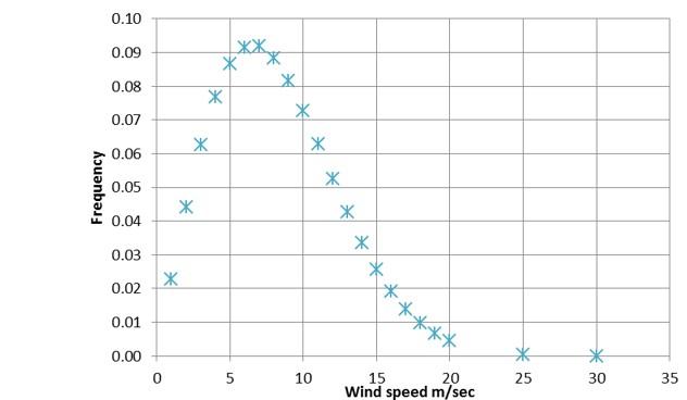
Figure A3-1. Site wind speed distribution.
Click for a full description
Figure A3.1 is a unimodal graph presenting the expected wind speed distribution for a site. It sets wind speed in metres per second - the x-function - against frequency of occurrence - the y-function. The graph demonstrates a probable proportional increase in frequency of wind speed up to approximately 7 metres per second with an exponential decrease to 25 metres per second.
Wind turbines usually operate with a range of operating rotor speeds between cut-in at the lowest wind speed enabling operation and maximum operating speed which is achieved when wind speed first enables full power to be generated. At increasing wind speeds above this operating wind speed, rotor speed is maintained at this maximum until at a high wind speed the turbine is shut down for protection, usually around 22-25m/sec. Between minimum and maximum rotor speeds, for simplicity it is assumed that rotor speed increases linearly with wind speed. Figure A3-2 indicates schematically how rotor speed varies with wind speed.
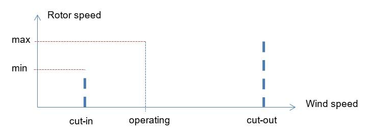
Figure A3-2. Rotor speed as a function of wind speed.
Click for a full description
Figure A3.2 is a schematic representation of rotor speed as a function of wind speeds. The horizontal function sets out three distinct stages of operation with increasing wind speed from left to right: cut-in, operating then cut-out. The vertical function represents the rotor speed in relation to these, with minimum operation coinciding with cut-in speeds and the maximum rotor speed coinciding with the operating stage. There is no coincidence between rotor speed and the cut-out wind speed.
The information available from the turbine manufacturer will usually specify an operational rotor speed range, a cut-in wind speed below which the rotor does not operate, a cut-out wind speed above which the turbine is shut down for protection and a rated wind speed which is the minimum wind speed at which the turbine will generate full power.
These two sets of data – wind speed frequency and rotor speed as a function of wind speed - must be brought together to calculate a mean rotor speed. Fig A3.3 shows both the site wind speed distribution, and the rotor speed (axis at right) as a function of wind speed for each of the two turbine options described in the worked example (Annex 1). For example, the manufacturer’s data for the 3.2 MW turbine indicates operating speeds in the range 6.7–12.1 rpm, with a cut-in wind speed of 3 m s-1, a cut-out wind speed of 22 m s-1 and rated wind speed (minimum wind speed generating full power) of 12 m s-1.
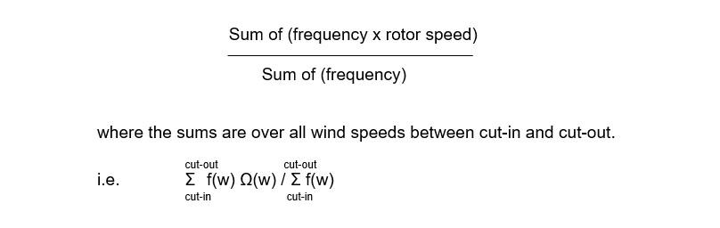
If a turbine has rotor speed Ω(w) at wind speed (w), and wind speed (w) occurs with frequency f(w), then the mean rotor speed is:
Equation A3-1
Click for a full description
Equation 3.1 calculates the mean rotor speed by dividing the sum of the frequency of the wind speed times the rotor speed by the frequency of the wind speed. This is explained in text and in mathematical format, i.e. between cut-in and cut-out speeds, sigma f(w) ohm(w) over sigma f(w).
The denominator is the proportion of time for which the wind speed is in operational range.
For the purpose of collision risk analysis it is sufficient to do this calculation by scaling off a graph like Figure A3-3, taking values for each frequency range of width one m/sec, e.g. from 7.5 m/sec to 8.5 m/sec. The accuracy of a graphical method is quite adequate within the context of the various other uncertainties in the calculation. (If desired, a more refined calculation may be done using a spreadsheet, an interpolation formula to evaluate the rotor speed at any given wind speed. A spreadsheet also facilitates comparison of a range of turbine options.)
Table 3.1 shows the results of scaling off Figure A3-3 for the 3.2 MW turbine. The second column reads wind speed frequency f(w) off the wind speed distribution, and the third column reads rotor speed Ω(w) off the rotor speed line. The final column calculates the mean rotor speed over operational time, taking the average of rotor speed weighted by frequency, as in equation (A3-1). It yields a mean rotor speed of 9.87 rpm for the 3.2 MW turbine used as an example.
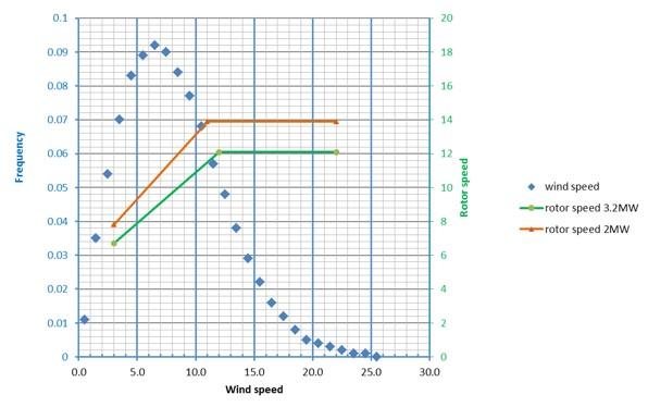
Figure A3-3. Bringing together wind frequency distribution and rotor speed data to calculate a mean rotor speed.
Click for a full description
This figure is a graphical overlay of information previously presented in Figure A3.1 (site wind speed distribution) and rotor speeds using an additional axis on the right, for two example turbines, i.e. 3.2MW and 2MW. The 3.2MW turbine is presented as a red line and the 2MW as a green line. The graph demonstrates proportionately lower rotor speeds for the 2MW turbine but both following a pattern of increasing to a point after which they plateau. Rotor speed lines above this wind speed remain horizontal.
Table A3-1. Calculation of mean rotor speed for 3.2MW turbine.
The wind speed frequency and rotor speed are read off from Figure A3-3.
Proportion of time wind speed is in operational range 3-22m/sec = 89.5
Mean rotor speed = 8.835 / 0.895 = 9.87 rpm
| Wind speed w | Wind speed frequency | Rotor speed | Product |
|---|---|---|---|
| 0-1 | 0.011 | - | - |
| 1-2 | 0.035 | Below cut-in | - |
| 2-3 | 0.054 | - | - |
| 3 – 4 | 0.070 | 7.0 | 0.490 |
| 4 – 5 | 0.083 | 7.6 | 0.631 |
| 5 – 6 | 0.089 | 8.2 | 0.730 |
| 6 – 7 | 0.092 | 8.8 | 0.810 |
| 7 – 8 | 0.090 | 9.4 | 0.846 |
| 8-9 | 0.084 | 10.0 | 0.840 |
| 9 – 10 | 0.077 | 10.6 | 0.816 |
| 10 – 11 | 0.068 | 11.2 | 0.762 |
| 11-12 | 0.057 | 11.8 | 0.673 |
| 12-13 | 0.048 | 12.1 | 0.581 |
| 13-14 | 0.038 | 12.1 | 0.460 |
| 14-15 | 0.029 | 12.1 | 0.351 |
| 15-16 | 0.022 | 12.1 | 0.266 |
| 16-17 | 0.016 | 12.1 | 0.194 |
| 17-18 | 0.012 | 12.1 | 0.145 |
| 18-19 | 0.008 | 12.1 | 0.097 |
| 19-20 | 0.005 | 12.1 | 0.061 |
| 20-21 | 0.004 | 12.1 | 0.048 |
| 21-22 | 0.003 | 12.1 | 0.036 |
| >22 | 0.000 | Above cut-out | - |
| Sum Σ f(w) | 0.895 | Sum Σ Ω (w) f(w) | 8.835 |
| Mean operational rotor speed Σ Ω (w) f(w) / Σ f(w) | - | - | 9.87 rpm |
Last updated: